
Forest Biomass Mapping
An end-to-end, multimodal pipeline that learns above-ground biomass density (AGBD) from sparse spaceborne lidar and turns it into wall-to-wall maps of Michigan. It fuses Sentinel-2 imagery and Google AlphaEarth embeddings, then splits biomass into leaf and wood using species-level allometry and phenology.
Code & trained weights: github.com/andrewh1001/forest-biomass-mapping · How to get the data
Tools: PyTorch, CNN + FiLM conditioning, GEDI L4A lidar, Sentinel-2, AlphaEarth embeddings, rasterio / GDAL, Google Earth Engine, MODIS LAI
| GEDI footprints (labels) | Output resolution | Test R² (total AGBD) | RMSE vs. mean predictor |
|---|---|---|---|
| 61,246 | 10 m | 0.78 | −53% (78.7 → 37.1 Mg/ha) |
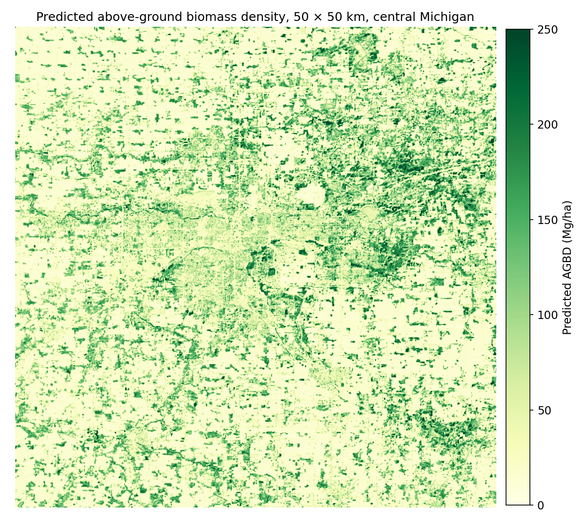 Figure 1. Predicted AGBD over a 50 × 50 km area of central Michigan. Woodlots, riparian corridors and larger forest blocks stand out against agricultural land and the urban core.
Overview
Forest biomass is central to carbon accounting, but measuring it directly is expensive. NASA’s GEDI lidar on the International Space Station estimates biomass very well, but only in scattered 25 m footprints along orbit tracks, and most of the land is never sampled. Optical satellites like Sentinel-2 see everything every few days, but can’t directly measure vertical structure.
This project trains a model to predict GEDI’s biomass from what Sentinel-2 and a learned Earth-observation embedding see around each footprint, then applies it to every 10 m pixel to produce continuous maps. A second stage asks a harder ecological question: how much of that biomass is leaves, and how much is wood?
Data
| Source | Role | Details |
|---|---|---|
| GEDI L4A (v2.1) | Labels | Footprint AGBD for 2024–2025, quality-filtered, within 350 km of central Michigan |
| Sentinel-2 L2A | Primary input | 10 bands as 21 × 21 px patches (210 m) per footprint; SCL cloud/snow masks; spring, summer and fall composites |
| AlphaEarth Foundations | Context input | 64-d annual (2024) embedding per location from Google Earth Engine |
| NLCD 2024 | Land cover | Forest type (deciduous, evergreen, mixed) and water masking |
| USFS TreeMap 2022 | Leaf prior | Per-pixel FIA plot imputation of tree species and stem density |
| BAAD + Jenkins et al. | Leaf prior | Measured and allometric leaf-to-total mass ratios per species |
| MODIS MCD15A2H | Validation | 8-day leaf area index, 2020–2026 |
 Figure 2. Sentinel-2 patches centered on GEDI footprints. Above roughly 50 Mg/ha, summer canopies look nearly identical in optical imagery, which is why the model needs spatial context and the AlphaEarth embedding, not just pixel spectra.
Pipeline
- Ingest: parse GEDI HDF5 beams, apply quality flags, download Sentinel-2 tiles and auxiliary rasters.
- Align: reproject everything to equal-area EPSG:6933, mosaic tiles, snap AlphaEarth onto the S2 grid.
- Sample: cut a 21 × 21 patch per footprint and drop no-data or cloudy patches.
- Train: ResNet-style fully convolutional network with AlphaEarth FiLM conditioning and a weighted log-space loss.
- Map: overlapping sliding-window inference over full scenes, written as cloud-masked 10 m GeoTIFFs.
- Prior: combine TreeMap species with BAAD and Jenkins ratios to get a per-pixel leaf fraction.
- Time series: predict 45 cloud-free dates from 2020–2026 and fit a two-term harmonic model.
- Validate: compare the seasonal leaf signal against MODIS LAI.
Model
The core network is a compact fully convolutional encoder over the Sentinel-2 patch. The AlphaEarth vector, plus per-patch snow and cloud fractions, conditions every stage through FiLM (feature-wise linear modulation), so the embedding shifts and scales the image features rather than being concatenated at the end. The FiLM layers are zero-initialized, so the network starts as a plain image model and learns how much to rely on the embedding. Biomass is read from the center pixel, which lets the same network run as a dense sliding-window map at inference time.
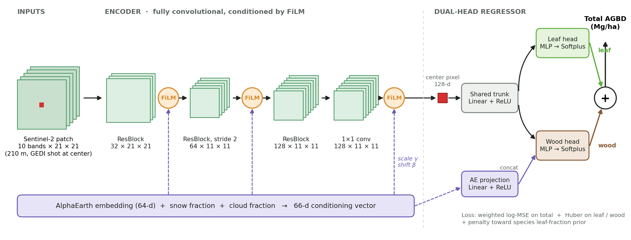 Figure 3. AlphaEarth conditions the image encoder through FiLM. The center-pixel feature feeds separate leaf and wood heads, whose sum is total AGBD.
Training details: AdamW (lr 1e-3, weight decay 3e-4) with reduce-on-plateau and gradient clipping. Because AGBD is heavily right-skewed (median 16, mean 63, max 575 Mg/ha), the loss is MSE in log space with extra weight on high-biomass samples. Hyperparameters were tuned with grid and Optuna searches.
Results
| Model | RMSE (Mg/ha) | RMSE ÷ target std | R² |
|---|---|---|---|
| Predict the mean | 78.7 | 1.00 | 0.00 |
| Random forest (canopy height, SRTM, Daymet, NLCD)* | 23.6 | 0.58 | 0.67 |
| CNN, S2 + AlphaEarth, single head | 37.6–39.7 | 0.48–0.50 | 0.75–0.77 |
| CNN, S2 + AlphaEarth, dual head | 37.1 | 0.47 | 0.78 |
*Scored on an earlier, smaller subset with a narrower biomass range (target std ≈ 41 vs. ≈ 79 Mg/ha), so compare R² or RMSE ÷ std rather than raw RMSE. On that scale the CNN’s error is about 20% lower relative to the spread of the data.
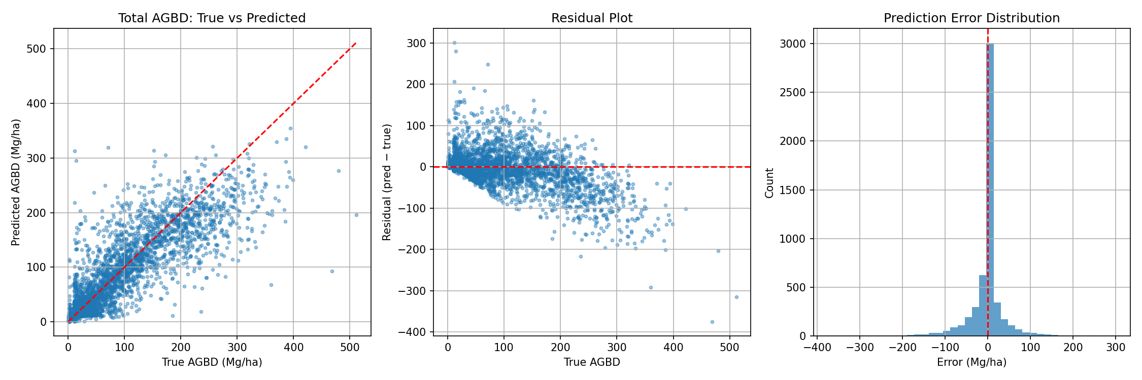 Figure 4. CNN on the held-out test set. Predictions follow the 1:1 line up to about 300 Mg/ha; very high-biomass stands are underestimated because optical signals saturate once the canopy closes.
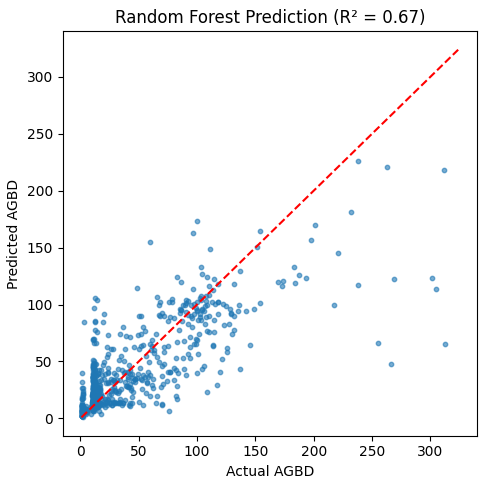 Figure 5. Random-forest baseline, which underestimates strongly above about 100 Mg/ha.
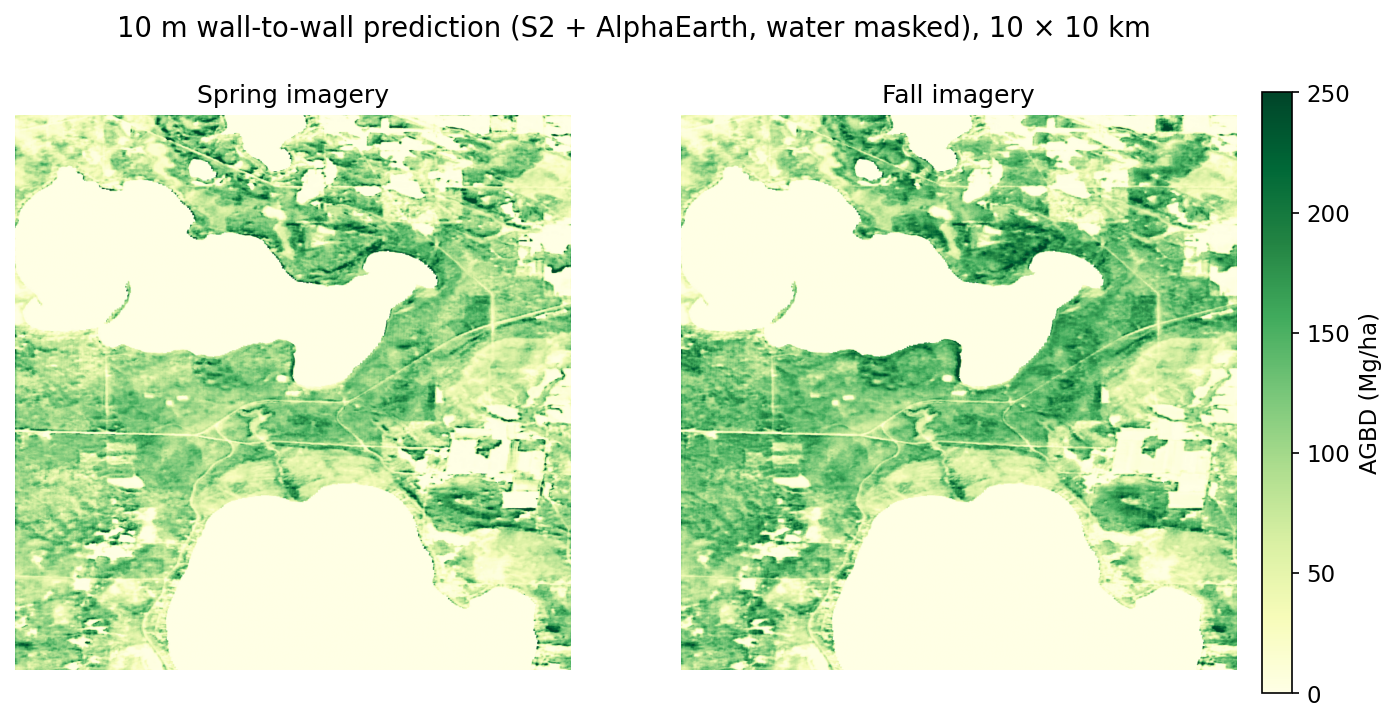 Figure 6. The same 10 km area mapped from spring and fall imagery: forest structure stays consistent across seasons.
Separating Leaves from Wood
Leaves cycle carbon every year, while wood stores it for decades. I explored two complementary ways to separate them.
Species-based leaf-fraction prior
For about 40 million forest pixels in Michigan, I looked up the TreeMap 2022 species list, weighted each species by stem density, and assigned a leaf-to-total mass ratio from BAAD where available and Jenkins et al. allometry otherwise.
| Forest type | Pixels | BAAD only | BAAD + Jenkins |
|---|---|---|---|
| Deciduous (NLCD 41) | 29.6 M | 0.150 | 0.084 ± 0.048 |
| Evergreen (NLCD 42) | 6.6 M | 0.230 | 0.124 ± 0.072 |
| Mixed (NLCD 43) | 4.3 M | 0.180 | 0.102 ± 0.060 |
Adding Jenkins allometry roughly halved the leaf fractions, since BAAD over-represents small and young trees.
Phenology from a 6-year time series
I ran the trained model on 45 cloud-free Sentinel-2 dates (2020–2026) over a deciduous study area and fit a two-term harmonic regression (R² = 0.77). The constant term is read as the wood component (≈145 Mg/ha) and the seasonal oscillation as leaf phenology, peaking around late July.
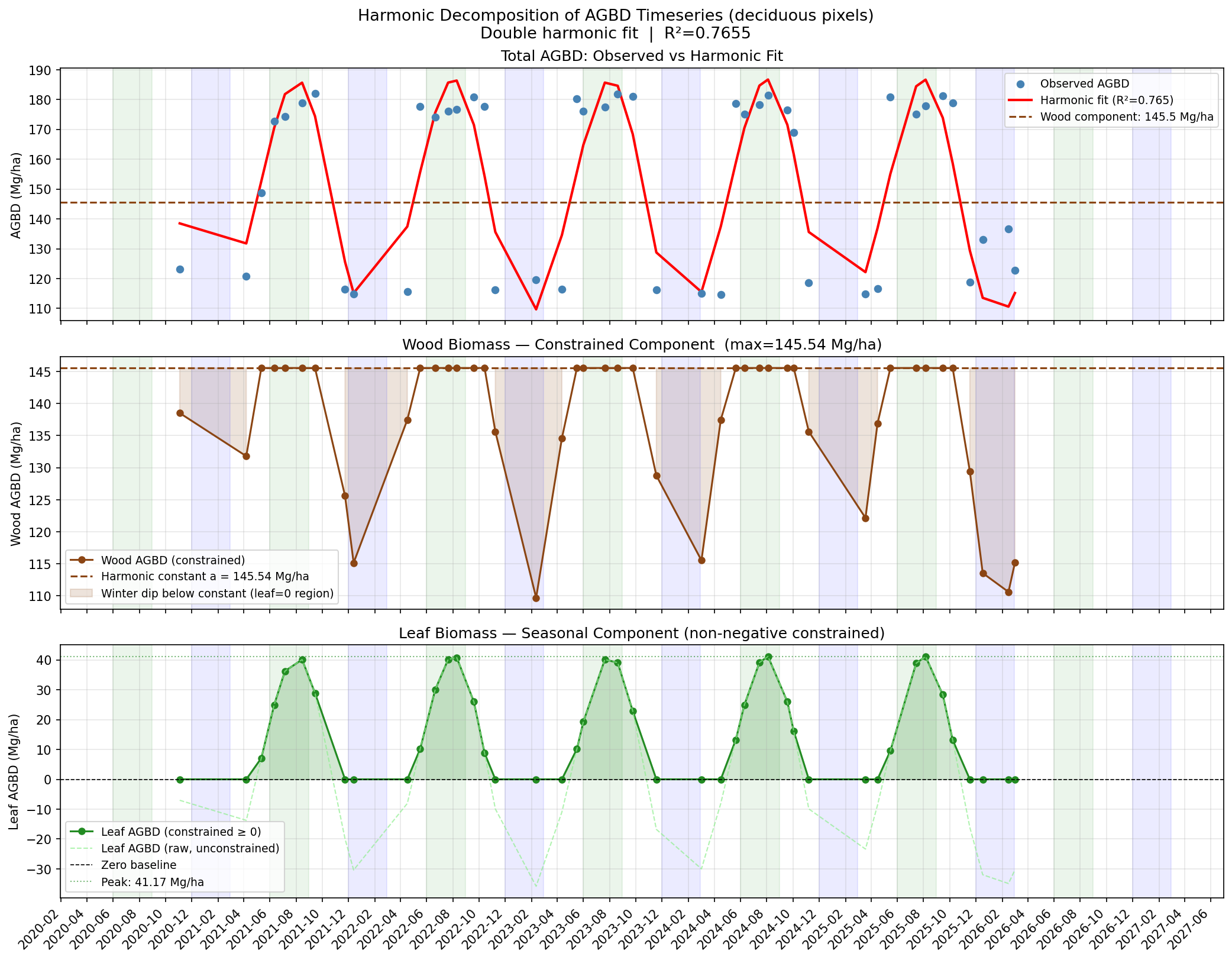 Figure 7. Harmonic decomposition of predicted AGBD into a constant wood component and a seasonal leaf component.
Compared with MODIS leaf area index over the same area, the seasonal leaf signal tracks closely (Pearson r = 0.87, Spearman ρ = 0.82), with green-up, peak and senescence lining up.
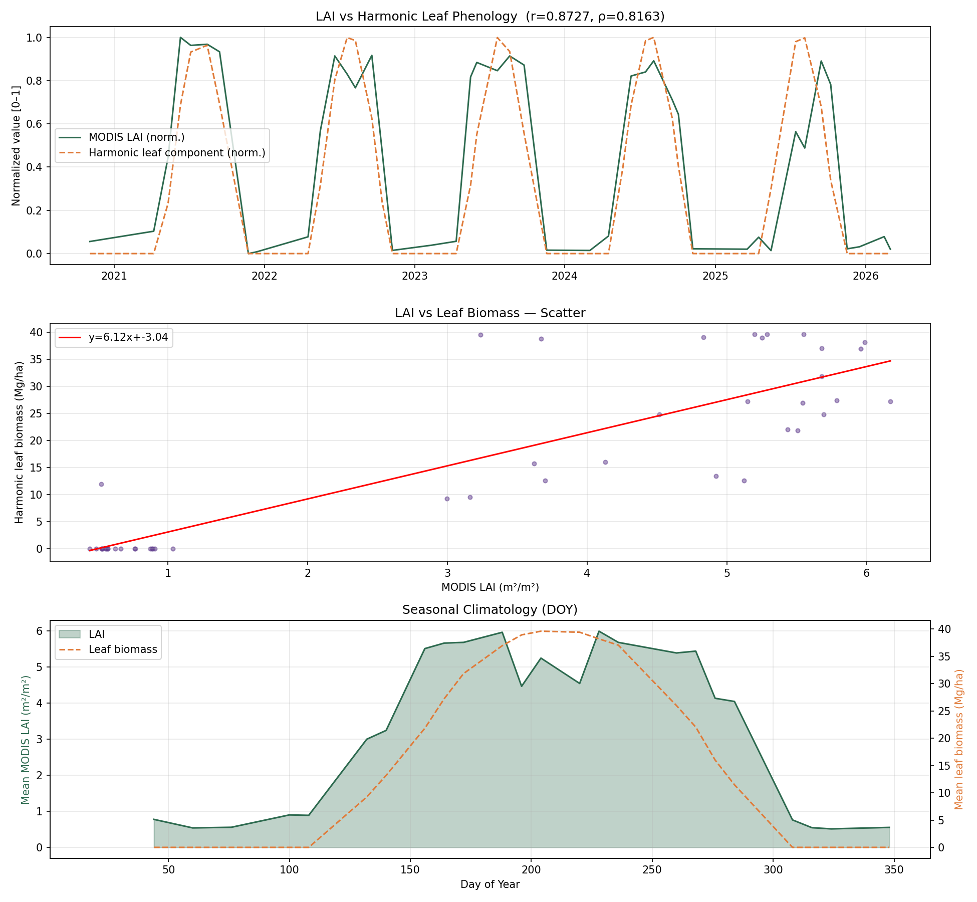 Figure 8. Validation against MODIS LAI: time series, scatter and seasonal climatology.
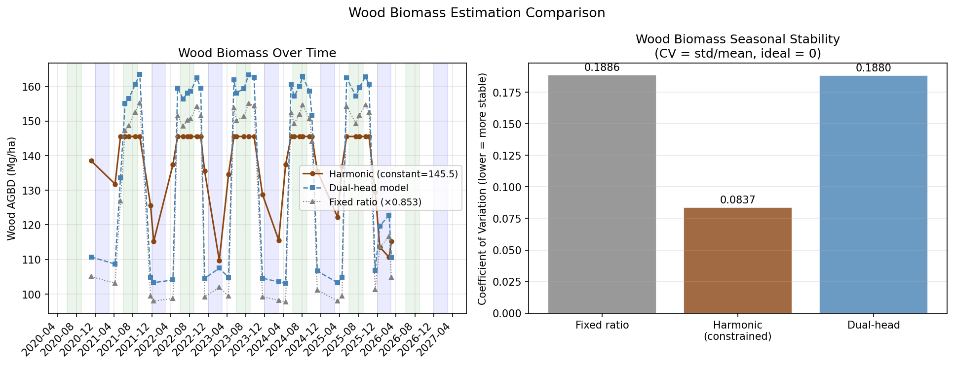 Figure 9. Wood biomass shouldn’t change with the seasons. The harmonic decomposition is the most stable (CV 0.084); fixed-ratio and dual-head approaches inherit the full seasonal swing (CV ≈ 0.19).
What I learned: the seasonal swing in predicted AGBD (about ±40 Mg/ha) is much larger than the foliage mass of a temperate forest, so the model partly responds to leaf-on/leaf-off reflectance changes. The LAI correlation confirms the signal is phenological, but it is better read as a canopy-greenness effect than literal leaf biomass.
Next Steps
- Spatial cross-validation by held-out orbit tracks or spatial blocks, since nearby GEDI shots have overlapping patches.
- Stratified metrics for forest pixels and by biomass bin, since half of the samples are under 20 Mg/ha.
- Ablations: S2-only vs. S2 + AlphaEarth, single- vs. multi-season inputs.
- Uncertainty: propagate GEDI L4A standard errors and ensemble variance into the maps.
Tech Stack
Python · PyTorch (CUDA) · rasterio · GDAL · geopandas · pyproj · h5py · xarray / rioxarray · scikit-learn · Optuna · NumPy / pandas · SciPy · Matplotlib · Google Earth Engine · NASA Earthdata / AppEEARS